Case Study
Nitrogen Source Optimization for Cellulase Production by Penicillium funiculosum, using a Sequential Experimental Design Methodology and the Desirability Function
The chosen article for the case study suggests employing a sequential experimental design methodology to enhance cellulase production efficiency. Lignocellulosic biomass, being one of the most abundant materials globally, holds immense potential for biomass production. However, the widespread application of lignocellulosic biomass for biofuel production faces constraints due to the considerable expenses associated with acquiring the necessary enzymes for the chemical process of deriving second-generation sugars. Consequently, the optimization of enzyme production emerges as a pivotal focus within the energy industry’s interests.
The Chosen Article
|
|---|
Second-generation ethanol production. Source: https://doi.org/10.1016/j.cej.2022.138690 |

Experimental Methods
Cellulase production by Penicillium funiculosum was assessed through the measurement of cellulase activity, quantified in terms of activity units (U), indicating the enzymatic extract required to liberate 1 μmol of sugars per minute.
Three distinct methods were employed to quantify cellulase activity, serving as the variables under consideration for optimization:
Filter Paper Assay (FPase)
Carboxymethylcellulose Assay (CMCase)
Cellobiose Assay (𝛽-Glucosidase)
The dependent variables in this study encompass the concentrations of various nitrogen sources present within the samples, namely:
Urea
Ammonium Sulfate
Peptone
Yeast Extract
The experimental samples consist of conical flasks, each containing 200 mL of a production medium. This medium features varying concentrations of urea, ammonium sulfate, peptone, and yeast extract, all acting as nitrogen sources. It’s worth noting that the carbon source remains constant throughout the experiments, maintaining a concentration of 15 g/L of partially delignified Cellulignin. Additionally, the spore suspension of Penicillium funiculosum ATCC 11797 maintains a consistent value of \(10^6\) conidia/mL.
Sequential Experimenta Design
|
|---|

The sequential experimental design involves a series of meticulously crafted iterations, wherein each step entails the elimination of an insignificant variable.
This systematic approach begins with a \(2^4\) factorial design, from which the least influential variable is identified and excluded based on Pareto plot analysis of the effects observed. The ensuing stage employs the remaining three variables within a \(2^3\) experimental design, following a similar process of identifying and omitting the least impactful variable. Ultimately, the final stage entails the execution of a central composite design, employing the last two variables that have emerged from the iterative refinement process.
Factorial \(2^4\)
|
|---|
Levels for independent variables for the \(2^4\) experimental design. |

|
|---|
Experimental results of each run of the \(2^4\) design. |

explann hands-on on \(2^4\) design
A python package (`explann <https://github.com/properallan/explann/>`__) was developed to assist design and statistical analysis of experiments.
All the following source code is hostes on github https://github.com/properallan/explann/. Both the table of levels and the experimental results can be easily imported to the explann package. There are functions to import data in string format or even xlsx file format. The explann package can assisti also in the creation of the experimetal design.
TwoLevelFactorial implements a generic \(2^n\) factorial design, with \(n\) variables defined as a dictionary containunt the variable name and range.
[1]:
from explann.doe import TwoLevelFactorial

f2b4 = TwoLevelFactorial(
    variables = {
        'U': (0.15, 0.45),
        'A': (0.70, 2.10),
        'P': (0.40, 1.10),
        'Y': (0.13, 0.38)
    },
    central_points=3
)
Once instantiated this class build the doe table, storage as an object attribute as a pandas DataFrame.
[2]:
f2b4.doe
[2]:
| U | A | P | Y | |
|---|---|---|---|---|
| Index | ||||
| 1 | -1.0 | -1.0 | -1.0 | -1.0 |
| 2 | 1.0 | -1.0 | -1.0 | -1.0 |
| 3 | -1.0 | 1.0 | -1.0 | -1.0 |
| 4 | 1.0 | 1.0 | -1.0 | -1.0 |
| 5 | -1.0 | -1.0 | 1.0 | -1.0 |
| 6 | 1.0 | -1.0 | 1.0 | -1.0 |
| 7 | -1.0 | 1.0 | 1.0 | -1.0 |
| 8 | 1.0 | 1.0 | 1.0 | -1.0 |
| 9 | -1.0 | -1.0 | -1.0 | 1.0 |
| 10 | 1.0 | -1.0 | -1.0 | 1.0 |
| 11 | -1.0 | 1.0 | -1.0 | 1.0 |
| 12 | 1.0 | 1.0 | -1.0 | 1.0 |
| 13 | -1.0 | -1.0 | 1.0 | 1.0 |
| 14 | 1.0 | -1.0 | 1.0 | 1.0 |
| 15 | -1.0 | 1.0 | 1.0 | 1.0 |
| 16 | 1.0 | 1.0 | 1.0 | 1.0 |
| 17 | 0.0 | 0.0 | 0.0 | 0.0 |
| 18 | 0.0 | 0.0 | 0.0 | 0.0 |
| 19 | 0.0 | 0.0 | 0.0 | 0.0 |
A table of the levels are also automaticly created.
[3]:
f2b4.levels
[3]:
| U | A | P | Y | |
|---|---|---|---|---|
| Levels | ||||
| -1.0 | 0.15 | 0.7 | 0.40 | 0.130 |
| 0.0 | 0.30 | 1.4 | 0.75 | 0.255 |
| 1.0 | 0.45 | 2.1 | 1.10 | 0.380 |
The doe table can be complemented with the response variables. For this task either ImportString or ImportXLSX can be used to load data.
[4]:
from explann.dataio import ImportString

f2b4_results = ImportString(data="""
F,CM,B
39,1.328,170
87,1.699,122
48,1.332,473
71,1.979,511
43,1.458,156
84,2.189,204
45,1.343,385
112,1.707,288
19,1.257,114
146,2.148,116
50,1.592,244
92,1.726,126
107,1.203,72
172,2.261,210
62,1.434,234
82,1.848,154
75,1.726,223
70,1.782,219
89,1.753,226
""",
delimiter=',')

f2b4_results.data
[4]:
| F | CM | B | |
|---|---|---|---|
| 1 | 39 | 1.328 | 170 |
| 2 | 87 | 1.699 | 122 |
| 3 | 48 | 1.332 | 473 |
| 4 | 71 | 1.979 | 511 |
| 5 | 43 | 1.458 | 156 |
| 6 | 84 | 2.189 | 204 |
| 7 | 45 | 1.343 | 385 |
| 8 | 112 | 1.707 | 288 |
| 9 | 19 | 1.257 | 114 |
| 10 | 146 | 2.148 | 116 |
| 11 | 50 | 1.592 | 244 |
| 12 | 92 | 1.726 | 126 |
| 13 | 107 | 1.203 | 72 |
| 14 | 172 | 2.261 | 210 |
| 15 | 62 | 1.434 | 234 |
| 16 | 82 | 1.848 | 154 |
| 17 | 75 | 1.726 | 223 |
| 18 | 70 | 1.782 | 219 |
| 19 | 89 | 1.753 | 226 |
The data is the merged with the doe table using append_results method.
[5]:
f2b4.append_results(results=f2b4_results.data)
f2b4.doe
[5]:
| U | A | P | Y | F | CM | B | |
|---|---|---|---|---|---|---|---|
| Index | |||||||
| 1 | -1.0 | -1.0 | -1.0 | -1.0 | 39 | 1.328 | 170 |
| 2 | 1.0 | -1.0 | -1.0 | -1.0 | 87 | 1.699 | 122 |
| 3 | -1.0 | 1.0 | -1.0 | -1.0 | 48 | 1.332 | 473 |
| 4 | 1.0 | 1.0 | -1.0 | -1.0 | 71 | 1.979 | 511 |
| 5 | -1.0 | -1.0 | 1.0 | -1.0 | 43 | 1.458 | 156 |
| 6 | 1.0 | -1.0 | 1.0 | -1.0 | 84 | 2.189 | 204 |
| 7 | -1.0 | 1.0 | 1.0 | -1.0 | 45 | 1.343 | 385 |
| 8 | 1.0 | 1.0 | 1.0 | -1.0 | 112 | 1.707 | 288 |
| 9 | -1.0 | -1.0 | -1.0 | 1.0 | 19 | 1.257 | 114 |
| 10 | 1.0 | -1.0 | -1.0 | 1.0 | 146 | 2.148 | 116 |
| 11 | -1.0 | 1.0 | -1.0 | 1.0 | 50 | 1.592 | 244 |
| 12 | 1.0 | 1.0 | -1.0 | 1.0 | 92 | 1.726 | 126 |
| 13 | -1.0 | -1.0 | 1.0 | 1.0 | 107 | 1.203 | 72 |
| 14 | 1.0 | -1.0 | 1.0 | 1.0 | 172 | 2.261 | 210 |
| 15 | -1.0 | 1.0 | 1.0 | 1.0 | 62 | 1.434 | 234 |
| 16 | 1.0 | 1.0 | 1.0 | 1.0 | 82 | 1.848 | 154 |
| 17 | 0.0 | 0.0 | 0.0 | 0.0 | 75 | 1.726 | 223 |
| 18 | 0.0 | 0.0 | 0.0 | 0.0 | 70 | 1.782 | 219 |
| 19 | 0.0 | 0.0 | 0.0 | 0.0 | 89 | 1.753 | 226 |
This experimental planning can be easily saved in .xlsx format. doe raw data is stored in the first sheet and the levels data is stored in a separate sheet named levels.
[6]:
f2b4.save_excel('../../data/f2b4.xlsx')
The ImporXLSX assist the import of data from excel file, this could be filled by hand or generated in explann as described above.
[7]:
from explann.dataio import ImportXLSX

f2b4_from_excel = ImportXLSX(
    path = '../../data/f2b4.xlsx',
    levels_sheet = 'levels'
)

f2b4_from_excel.data
[7]:
| Index | U | A | P | Y | F | CM | B | |
|---|---|---|---|---|---|---|---|---|
| 1 | 1 | -1 | -1 | -1 | -1 | 39 | 1.328 | 170 |
| 2 | 2 | 1 | -1 | -1 | -1 | 87 | 1.699 | 122 |
| 3 | 3 | -1 | 1 | -1 | -1 | 48 | 1.332 | 473 |
| 4 | 4 | 1 | 1 | -1 | -1 | 71 | 1.979 | 511 |
| 5 | 5 | -1 | -1 | 1 | -1 | 43 | 1.458 | 156 |
| 6 | 6 | 1 | -1 | 1 | -1 | 84 | 2.189 | 204 |
| 7 | 7 | -1 | 1 | 1 | -1 | 45 | 1.343 | 385 |
| 8 | 8 | 1 | 1 | 1 | -1 | 112 | 1.707 | 288 |
| 9 | 9 | -1 | -1 | -1 | 1 | 19 | 1.257 | 114 |
| 10 | 10 | 1 | -1 | -1 | 1 | 146 | 2.148 | 116 |
| 11 | 11 | -1 | 1 | -1 | 1 | 50 | 1.592 | 244 |
| 12 | 12 | 1 | 1 | -1 | 1 | 92 | 1.726 | 126 |
| 13 | 13 | -1 | -1 | 1 | 1 | 107 | 1.203 | 72 |
| 14 | 14 | 1 | -1 | 1 | 1 | 172 | 2.261 | 210 |
| 15 | 15 | -1 | 1 | 1 | 1 | 62 | 1.434 | 234 |
| 16 | 16 | 1 | 1 | 1 | 1 | 82 | 1.848 | 154 |
| 17 | 17 | 0 | 0 | 0 | 0 | 75 | 1.726 | 223 |
| 18 | 18 | 0 | 0 | 0 | 0 | 70 | 1.782 | 219 |
| 19 | 19 | 0 | 0 | 0 | 0 | 89 | 1.753 | 226 |
If the levels_sheet argument is passed, the loaded object will contain an aditional table with the levels parsed.
[8]:
f2b4_from_excel.parsed_data
[8]:
| Index | U | A | P | Y | F | CM | B | |
|---|---|---|---|---|---|---|---|---|
| 1 | 1 | 0.45 | 0.7 | 0.40 | 0.130 | 39 | 1.328 | 170 |
| 2 | 2 | 0.15 | 2.1 | 0.40 | 0.130 | 87 | 1.699 | 122 |
| 3 | 3 | 0.45 | 2.1 | 0.40 | 0.130 | 48 | 1.332 | 473 |
| 4 | 4 | 0.15 | 0.7 | 1.10 | 0.130 | 71 | 1.979 | 511 |
| 5 | 5 | 0.45 | 0.7 | 1.10 | 0.130 | 43 | 1.458 | 156 |
| 6 | 6 | 0.15 | 2.1 | 1.10 | 0.130 | 84 | 2.189 | 204 |
| 7 | 7 | 0.45 | 2.1 | 1.10 | 0.130 | 45 | 1.343 | 385 |
| 8 | 8 | 0.15 | 0.7 | 0.40 | 0.380 | 112 | 1.707 | 288 |
| 9 | 9 | 0.45 | 0.7 | 0.40 | 0.380 | 19 | 1.257 | 114 |
| 10 | 10 | 0.15 | 2.1 | 0.40 | 0.380 | 146 | 2.148 | 116 |
| 11 | 11 | 0.45 | 2.1 | 0.40 | 0.380 | 50 | 1.592 | 244 |
| 12 | 12 | 0.15 | 0.7 | 1.10 | 0.380 | 92 | 1.726 | 126 |
| 13 | 13 | 0.45 | 0.7 | 1.10 | 0.380 | 107 | 1.203 | 72 |
| 14 | 14 | 0.15 | 2.1 | 1.10 | 0.380 | 172 | 2.261 | 210 |
| 15 | 15 | 0.45 | 2.1 | 1.10 | 0.380 | 62 | 1.434 | 234 |
| 16 | 16 | 0.30 | 1.4 | 0.75 | 0.255 | 82 | 1.848 | 154 |
| 17 | 17 | 0.30 | 1.4 | 0.75 | 0.255 | 75 | 1.726 | 223 |
| 18 | 18 | 0.30 | 1.4 | 0.75 | 0.255 | 70 | 1.782 | 219 |
| 19 | 19 | 0.00 | 0.0 | 0.00 | 0.000 | 89 | 1.753 | 226 |
We can now use the data to build our factorial model. The functions attribute is a dictionary, the keys are funcion names, and the values are function equations, the syntax follows `patsy <https://patsy.readthedocs.io/en/latest/>`__ stardadization. Here U * A * P * Y stands for all interaction terms between the 4 variables
[9]:
from explann.models import FactorialModel

fm2b4 = FactorialModel(
    data = f2b4_from_excel.data,
    functions = {
        "Fso"  : "F ~ U * A * P * Y + I(U**2) + I(A**2) + I(P**2) + I(Y**2)",
        "CMso" : "CM ~ U * A * P * Y + I(U**2) + I(A**2) + I(P**2) + I(Y**2)",
        "Bso"  : "B ~ U * A * P * Y + I(U**2) + I(A**2) + I(P**2) + I(Y**2)",
        "F"  : "F ~ U * A * P * Y",
        "CM" : "CM ~ U * A * P * Y",
        "B"  : "B ~ U * A * P * Y"}
)
The object fm2b4 stores all the filted models(Ordinary Least Squares) listed in functions, any given model can be retriev by indexing by function name.
[10]:
fm2b4['F']
[10]:
<statsmodels.regression.linear_model.RegressionResultsWrapper at 0x7fcd1570edf0>
An overview of the results can be viewd using the summary method. The method accepts also a given funtion name as argument, if None is passed a dictionary of summary() is returned.
[11]:
fm2b4.summary()
/home/ppiper/micromamba/envs/explann/lib/python3.9/site-packages/scipy/stats/_stats_py.py:1806: UserWarning: kurtosistest only valid for n>=20 ... continuing anyway, n=19
  warnings.warn("kurtosistest only valid for n>=20 ... continuing "
/home/ppiper/micromamba/envs/explann/lib/python3.9/site-packages/scipy/stats/_stats_py.py:1806: UserWarning: kurtosistest only valid for n>=20 ... continuing anyway, n=19
  warnings.warn("kurtosistest only valid for n>=20 ... continuing "
/home/ppiper/micromamba/envs/explann/lib/python3.9/site-packages/scipy/stats/_stats_py.py:1806: UserWarning: kurtosistest only valid for n>=20 ... continuing anyway, n=19
  warnings.warn("kurtosistest only valid for n>=20 ... continuing "
/home/ppiper/micromamba/envs/explann/lib/python3.9/site-packages/scipy/stats/_stats_py.py:1806: UserWarning: kurtosistest only valid for n>=20 ... continuing anyway, n=19
  warnings.warn("kurtosistest only valid for n>=20 ... continuing "
/home/ppiper/micromamba/envs/explann/lib/python3.9/site-packages/scipy/stats/_stats_py.py:1806: UserWarning: kurtosistest only valid for n>=20 ... continuing anyway, n=19
  warnings.warn("kurtosistest only valid for n>=20 ... continuing "
/home/ppiper/micromamba/envs/explann/lib/python3.9/site-packages/scipy/stats/_stats_py.py:1806: UserWarning: kurtosistest only valid for n>=20 ... continuing anyway, n=19
  warnings.warn("kurtosistest only valid for n>=20 ... continuing "
[11]:
{'Fso': <class 'statsmodels.iolib.summary.Summary'>
"""
OLS Regression Results
==============================================================================
Dep. Variable: F R-squared: 0.992
Model: OLS Adj. R-squared: 0.931
Method: Least Squares F-statistic: 16.16
Date: Wed, 16 Aug 2023 Prob (F-statistic): 0.0598
Time: 19:16:43 Log-Likelihood: -49.032
No. Observations: 19 AIC: 132.1
Df Residuals: 2 BIC: 148.1
Df Model: 16
Covariance Type: nonrobust
==============================================================================
coef std err t P>|t| [0.025 0.975]
------------------------------------------------------------------------------
Intercept 78.0000 5.686 13.717 0.005 53.534 102.466
U 27.0625 2.462 10.991 0.008 16.468 37.657
A -8.4375 2.462 -3.427 0.076 -19.032 2.157
U:A -8.0625 2.462 -3.274 0.082 -18.657 2.532
P 9.6875 2.462 3.934 0.059 -0.907 20.282
U:P -2.9375 2.462 -1.193 0.355 -13.532 7.657
A:P -4.6875 2.462 -1.904 0.197 -15.282 5.907
U:A:P 5.6875 2.462 2.310 0.147 -4.907 16.282
Y 12.5625 2.462 5.102 0.036 1.968 23.157
U:Y 4.6875 2.462 1.904 0.197 -5.907 15.282
A:Y -11.3125 2.462 -4.594 0.044 -21.907 -0.718
U:A:Y -8.1875 2.462 -3.325 0.080 -18.782 2.407
P:Y 4.8125 2.462 1.955 0.190 -5.782 15.407
U:P:Y -7.5625 2.462 -3.071 0.092 -18.157 3.032
A:P:Y -9.3125 2.462 -3.782 0.063 -19.907 1.282
U:A:P:Y -0.6875 2.462 -0.279 0.806 -11.282 9.907
I(U ** 2) 0.1719 1.549 0.111 0.922 -6.493 6.837
I(A ** 2) 0.1719 1.549 0.111 0.922 -6.493 6.837
I(P ** 2) 0.1719 1.549 0.111 0.922 -6.493 6.837
I(Y ** 2) 0.1719 1.549 0.111 0.922 -6.493 6.837
==============================================================================
Omnibus: 19.262 Durbin-Watson: 2.036
Prob(Omnibus): 0.000 Jarque-Bera (JB): 38.617
Skew: 1.278 Prob(JB): 4.12e-09
Kurtosis: 9.500 Cond. No. 1.96e+30
==============================================================================
Notes:
[1] Standard Errors assume that the covariance matrix of the errors is correctly specified.
[2] The input rank is higher than the number of observations.
[3] The smallest eigenvalue is 2.1e-59. This might indicate that there are
strong multicollinearity problems or that the design matrix is singular.
""",
'CMso': <class 'statsmodels.iolib.summary.Summary'>
"""
OLS Regression Results
==============================================================================
Dep. Variable: CM R-squared: 0.999
Model: OLS Adj. R-squared: 0.992
Method: Least Squares F-statistic: 146.2
Date: Wed, 16 Aug 2023 Prob (F-statistic): 0.00682
Time: 19:16:43 Log-Likelihood: 62.359
No. Observations: 19 AIC: -90.72
Df Residuals: 2 BIC: -74.66
Df Model: 16
Covariance Type: nonrobust
==============================================================================
coef std err t P>|t| [0.025 0.975]
------------------------------------------------------------------------------
Intercept 1.7537 0.016 108.457 0.000 1.684 1.823
U 0.2881 0.007 41.152 0.001 0.258 0.318
A -0.0364 0.007 -5.195 0.035 -0.066 -0.006
U:A -0.0933 0.007 -13.319 0.006 -0.123 -0.063
P 0.0239 0.007 3.410 0.076 -0.006 0.054
U:P 0.0327 0.007 4.678 0.043 0.003 0.063
A:P -0.0610 0.007 -8.712 0.013 -0.091 -0.031
U:A:P -0.0331 0.007 -4.731 0.042 -0.063 -0.003
Y 0.0271 0.007 3.874 0.061 -0.003 0.057
U:Y 0.0240 0.007 3.428 0.076 -0.006 0.054
A:Y 0.0027 0.007 0.393 0.732 -0.027 0.033
U:A:Y -0.0819 0.007 -11.694 0.007 -0.112 -0.052
P:Y -0.0210 0.007 -2.999 0.096 -0.051 0.009
U:P:Y 0.0231 0.007 3.303 0.081 -0.007 0.053
A:P:Y 0.0491 0.007 7.016 0.020 0.019 0.079
U:A:P:Y 0.0472 0.007 6.749 0.021 0.017 0.077
I(U ** 2) -0.0243 0.004 -5.515 0.031 -0.043 -0.005
I(A ** 2) -0.0243 0.004 -5.515 0.031 -0.043 -0.005
I(P ** 2) -0.0243 0.004 -5.515 0.031 -0.043 -0.005
I(Y ** 2) -0.0243 0.004 -5.515 0.031 -0.043 -0.005
==============================================================================
Omnibus: 13.078 Durbin-Watson: 3.023
Prob(Omnibus): 0.001 Jarque-Bera (JB): 33.486
Skew: 0.110 Prob(JB): 5.35e-08
Kurtosis: 9.500 Cond. No. 1.96e+30
==============================================================================
Notes:
[1] Standard Errors assume that the covariance matrix of the errors is correctly specified.
[2] The input rank is higher than the number of observations.
[3] The smallest eigenvalue is 2.1e-59. This might indicate that there are
strong multicollinearity problems or that the design matrix is singular.
""",
'Bso': <class 'statsmodels.iolib.summary.Summary'>
"""
OLS Regression Results
==============================================================================
Dep. Variable: B R-squared: 1.000
Model: OLS Adj. R-squared: 0.999
Method: Least Squares F-statistic: 1291.
Date: Wed, 16 Aug 2023 Prob (F-statistic): 0.000774
Time: 19:16:43 Log-Likelihood: -29.439
No. Observations: 19 AIC: 92.88
Df Residuals: 2 BIC: 108.9
Df Model: 16
Covariance Type: nonrobust
==============================================================================
coef std err t P>|t| [0.025 0.975]
------------------------------------------------------------------------------
Intercept 222.6667 2.028 109.819 0.000 213.943 231.391
U -7.3125 0.878 -8.329 0.014 -11.090 -3.535
A 78.1875 0.878 89.055 0.000 74.410 81.965
U:A -24.8125 0.878 -28.261 0.001 -28.590 -21.035
P -10.8125 0.878 -12.315 0.007 -14.590 -7.035
U:P 8.4375 0.878 9.610 0.011 4.660 12.215
A:P -25.8125 0.878 -29.400 0.001 -29.590 -22.035
U:A:P -20.5625 0.878 -23.420 0.002 -24.340 -16.785
Y -64.9375 0.878 -73.963 0.000 -68.715 -61.160
U:Y 0.0625 0.878 0.071 0.950 -3.715 3.840
A:Y -47.4375 0.878 -54.031 0.000 -51.215 -43.660
U:A:Y -17.4375 0.878 -19.861 0.003 -21.215 -13.660
P:Y 19.5625 0.878 22.281 0.002 15.785 23.340
U:P:Y 13.3125 0.878 15.163 0.004 9.535 17.090
A:P:Y 21.5625 0.878 24.559 0.002 17.785 25.340
U:A:P:Y 8.3125 0.878 9.468 0.011 4.535 12.090
I(U ** 2) 0.2552 0.552 0.462 0.689 -2.121 2.632
I(A ** 2) 0.2552 0.552 0.462 0.689 -2.121 2.632
I(P ** 2) 0.2552 0.552 0.462 0.689 -2.121 2.632
I(Y ** 2) 0.2552 0.552 0.462 0.689 -2.121 2.632
==============================================================================
Omnibus: 13.909 Durbin-Watson: 2.640
Prob(Omnibus): 0.001 Jarque-Bera (JB): 34.047
Skew: -0.435 Prob(JB): 4.04e-08
Kurtosis: 9.500 Cond. No. 1.96e+30
==============================================================================
Notes:
[1] Standard Errors assume that the covariance matrix of the errors is correctly specified.
[2] The input rank is higher than the number of observations.
[3] The smallest eigenvalue is 2.1e-59. This might indicate that there are
strong multicollinearity problems or that the design matrix is singular.
""",
'F': <class 'statsmodels.iolib.summary.Summary'>
"""
OLS Regression Results
==============================================================================
Dep. Variable: F R-squared: 0.992
Model: OLS Adj. R-squared: 0.954
Method: Least Squares F-statistic: 25.70
Date: Wed, 16 Aug 2023 Prob (F-statistic): 0.0107
Time: 19:16:43 Log-Likelihood: -49.091
No. Observations: 19 AIC: 130.2
Df Residuals: 3 BIC: 145.3
Df Model: 15
Covariance Type: nonrobust
==============================================================================
coef std err t P>|t| [0.025 0.975]
------------------------------------------------------------------------------
Intercept 78.5789 1.851 42.463 0.000 72.690 84.468
U 27.0625 2.017 13.420 0.001 20.645 33.480
A -8.4375 2.017 -4.184 0.025 -14.855 -2.020
U:A -8.0625 2.017 -3.998 0.028 -14.480 -1.645
P 9.6875 2.017 4.804 0.017 3.270 16.105
U:P -2.9375 2.017 -1.457 0.241 -9.355 3.480
A:P -4.6875 2.017 -2.324 0.103 -11.105 1.730
U:A:P 5.6875 2.017 2.820 0.067 -0.730 12.105
Y 12.5625 2.017 6.230 0.008 6.145 18.980
U:Y 4.6875 2.017 2.324 0.103 -1.730 11.105
A:Y -11.3125 2.017 -5.610 0.011 -17.730 -4.895
U:A:Y -8.1875 2.017 -4.060 0.027 -14.605 -1.770
P:Y 4.8125 2.017 2.386 0.097 -1.605 11.230
U:P:Y -7.5625 2.017 -3.750 0.033 -13.980 -1.145
A:P:Y -9.3125 2.017 -4.618 0.019 -15.730 -2.895
U:A:P:Y -0.6875 2.017 -0.341 0.756 -7.105 5.730
==============================================================================
Omnibus: 14.090 Durbin-Watson: 2.047
Prob(Omnibus): 0.001 Jarque-Bera (JB): 27.071
Skew: 0.726 Prob(JB): 1.32e-06
Kurtosis: 8.664 Cond. No. 1.09
==============================================================================
Notes:
[1] Standard Errors assume that the covariance matrix of the errors is correctly specified.
""",
'CM': <class 'statsmodels.iolib.summary.Summary'>
"""
OLS Regression Results
==============================================================================
Dep. Variable: CM R-squared: 0.986
Model: OLS Adj. R-squared: 0.917
Method: Least Squares F-statistic: 14.24
Date: Wed, 16 Aug 2023 Prob (F-statistic): 0.0250
Time: 19:16:43 Log-Likelihood: 35.898
No. Observations: 19 AIC: -39.80
Df Residuals: 3 BIC: -24.69
Df Model: 15
Covariance Type: nonrobust
==============================================================================
coef std err t P>|t| [0.025 0.975]
------------------------------------------------------------------------------
Intercept 1.6718 0.021 79.166 0.000 1.605 1.739
U 0.2881 0.023 12.520 0.001 0.215 0.361
A -0.0364 0.023 -1.581 0.212 -0.110 0.037
U:A -0.0932 0.023 -4.052 0.027 -0.166 -0.020
P 0.0239 0.023 1.037 0.376 -0.049 0.097
U:P 0.0328 0.023 1.423 0.250 -0.040 0.106
A:P -0.0610 0.023 -2.651 0.077 -0.134 0.012
U:A:P -0.0331 0.023 -1.439 0.246 -0.106 0.040
Y 0.0271 0.023 1.179 0.323 -0.046 0.100
U:Y 0.0240 0.023 1.043 0.374 -0.049 0.097
A:Y 0.0028 0.023 0.119 0.912 -0.070 0.076
U:A:Y -0.0819 0.023 -3.558 0.038 -0.155 -0.009
P:Y -0.0210 0.023 -0.913 0.429 -0.094 0.052
U:P:Y 0.0231 0.023 1.005 0.389 -0.050 0.096
A:P:Y 0.0491 0.023 2.135 0.122 -0.024 0.122
U:A:P:Y 0.0473 0.023 2.053 0.132 -0.026 0.120
==============================================================================
Omnibus: 19.927 Durbin-Watson: 0.346
Prob(Omnibus): 0.000 Jarque-Bera (JB): 20.834
Skew: 2.121 Prob(JB): 2.99e-05
Kurtosis: 5.884 Cond. No. 1.09
==============================================================================
Notes:
[1] Standard Errors assume that the covariance matrix of the errors is correctly specified.
""",
'B': <class 'statsmodels.iolib.summary.Summary'>
"""
OLS Regression Results
==============================================================================
Dep. Variable: B R-squared: 1.000
Model: OLS Adj. R-squared: 0.999
Method: Least Squares F-statistic: 1867.
Date: Wed, 16 Aug 2023 Prob (F-statistic): 1.80e-05
Time: 19:16:43 Log-Likelihood: -30.403
No. Observations: 19 AIC: 92.81
Df Residuals: 3 BIC: 107.9
Df Model: 15
Covariance Type: nonrobust
==============================================================================
coef std err t P>|t| [0.025 0.975]
------------------------------------------------------------------------------
Intercept 223.5263 0.692 322.991 0.000 221.324 225.729
U -7.3125 0.754 -9.696 0.002 -9.713 -4.912
A 78.1875 0.754 103.677 0.000 75.787 80.588
U:A -24.8125 0.754 -32.901 0.000 -27.213 -22.412
P -10.8125 0.754 -14.337 0.001 -13.213 -8.412
U:P 8.4375 0.754 11.188 0.002 6.037 10.838
A:P -25.8125 0.754 -34.227 0.000 -28.213 -23.412
U:A:P -20.5625 0.754 -27.266 0.000 -22.963 -18.162
Y -64.9375 0.754 -86.107 0.000 -67.338 -62.537
U:Y 0.0625 0.754 0.083 0.939 -2.338 2.463
A:Y -47.4375 0.754 -62.902 0.000 -49.838 -45.037
U:A:Y -17.4375 0.754 -23.122 0.000 -19.838 -15.037
P:Y 19.5625 0.754 25.940 0.000 17.162 21.963
U:P:Y 13.3125 0.754 17.652 0.000 10.912 15.713
A:P:Y 21.5625 0.754 28.592 0.000 19.162 23.963
U:A:P:Y 8.3125 0.754 11.022 0.002 5.912 10.713
==============================================================================
Omnibus: 31.293 Durbin-Watson: 2.398
Prob(Omnibus): 0.000 Jarque-Bera (JB): 77.186
Skew: -2.374 Prob(JB): 1.73e-17
Kurtosis: 11.658 Cond. No. 1.09
==============================================================================
Notes:
[1] Standard Errors assume that the covariance matrix of the errors is correctly specified.
"""}
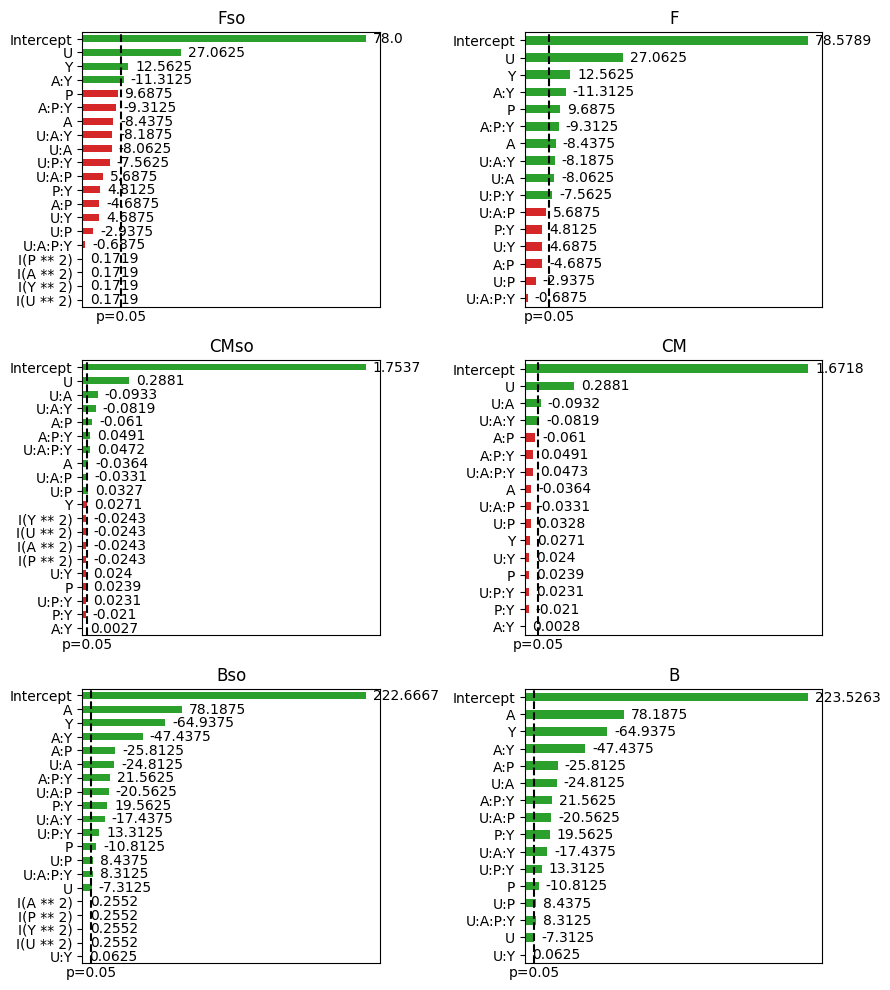
[12]:
from explann.plot import ParetoPlot

import matplotlib.pyplot as plt
fig, ax = plt.subplots(3,2, figsize=(9,10))
ax = ax.flatten()
pp_fm2b4 = ParetoPlot(fm2b4)

pp_fm2b4.plot(['Fso', 'F', 'CMso', 'CM' ,'Bso', 'B'], ax=ax)
plt.tight_layout()

[13]:
fm2b4.print_equation()
[13]:
{'Fso': 'F = 78.0000 + 27.0625 * U + 12.5625 * Y - 11.3125 * AY',
 'CMso': 'CM = 1.7537 + 0.2881 * U - 0.0364 * A - 0.0933 * UA + 0.0327 * UP - 0.0610 * AP - 0.0331 * UAP - 0.0819 * UAY + 0.0491 * APY + 0.0472 * UAPY - 0.0243 * I(U ** 2) - 0.0243 * I(A ** 2) - 0.0243 * I(P ** 2) - 0.0243 * I(Y ** 2)',
 'Bso': 'B = 222.6667 - 7.3125 * U + 78.1875 * A - 24.8125 * UA - 10.8125 * P + 8.4375 * UP - 25.8125 * AP - 20.5625 * UAP - 64.9375 * Y - 47.4375 * AY - 17.4375 * UAY + 19.5625 * PY + 13.3125 * UPY + 21.5625 * APY + 8.3125 * UAPY',
 'F': 'F = 78.5789 + 27.0625 * U - 8.4375 * A - 8.0625 * UA + 9.6875 * P + 12.5625 * Y - 11.3125 * AY - 8.1875 * UAY - 7.5625 * UPY - 9.3125 * APY',
 'CM': 'CM = 1.6718 + 0.2881 * U - 0.0932 * UA - 0.0819 * UAY',
 'B': 'B = 223.5263 - 7.3125 * U + 78.1875 * A - 24.8125 * UA - 10.8125 * P + 8.4375 * UP - 25.8125 * AP - 20.5625 * UAP - 64.9375 * Y - 47.4375 * AY - 17.4375 * UAY + 19.5625 * PY + 13.3125 * UPY + 21.5625 * APY + 8.3125 * UAPY'}
build_significant_models get the models with only significant terms withing a significance value \(\alpha\).
[14]:
sig_fm2b4=fm2b4.build_significant_models(alpha=0.05)
sig_fm2b4.summary()
/home/ppiper/micromamba/envs/explann/lib/python3.9/site-packages/scipy/stats/_stats_py.py:1806: UserWarning: kurtosistest only valid for n>=20 ... continuing anyway, n=19
  warnings.warn("kurtosistest only valid for n>=20 ... continuing "
/home/ppiper/micromamba/envs/explann/lib/python3.9/site-packages/scipy/stats/_stats_py.py:1806: UserWarning: kurtosistest only valid for n>=20 ... continuing anyway, n=19
  warnings.warn("kurtosistest only valid for n>=20 ... continuing "
/home/ppiper/micromamba/envs/explann/lib/python3.9/site-packages/scipy/stats/_stats_py.py:1806: UserWarning: kurtosistest only valid for n>=20 ... continuing anyway, n=19
  warnings.warn("kurtosistest only valid for n>=20 ... continuing "
/home/ppiper/micromamba/envs/explann/lib/python3.9/site-packages/scipy/stats/_stats_py.py:1806: UserWarning: kurtosistest only valid for n>=20 ... continuing anyway, n=19
  warnings.warn("kurtosistest only valid for n>=20 ... continuing "
/home/ppiper/micromamba/envs/explann/lib/python3.9/site-packages/scipy/stats/_stats_py.py:1806: UserWarning: kurtosistest only valid for n>=20 ... continuing anyway, n=19
  warnings.warn("kurtosistest only valid for n>=20 ... continuing "
/home/ppiper/micromamba/envs/explann/lib/python3.9/site-packages/scipy/stats/_stats_py.py:1806: UserWarning: kurtosistest only valid for n>=20 ... continuing anyway, n=19
  warnings.warn("kurtosistest only valid for n>=20 ... continuing "
[14]:
{'Fso': <class 'statsmodels.iolib.summary.Summary'>
"""
OLS Regression Results
==============================================================================
Dep. Variable: F R-squared: 0.644
Model: OLS Adj. R-squared: 0.573
Method: Least Squares F-statistic: 9.063
Date: Wed, 16 Aug 2023 Prob (F-statistic): 0.00115
Time: 19:16:45 Log-Likelihood: -85.472
No. Observations: 19 AIC: 178.9
Df Residuals: 15 BIC: 182.7
Df Model: 3
Covariance Type: nonrobust
==============================================================================
coef std err t P>|t| [0.025 0.975]
------------------------------------------------------------------------------
Intercept 78.5789 5.616 13.993 0.000 66.609 90.549
U 27.0625 6.120 4.422 0.000 14.019 40.106
Y 12.5625 6.120 2.053 0.058 -0.481 25.606
A:Y -11.3125 6.120 -1.849 0.084 -24.356 1.731
==============================================================================
Omnibus: 3.592 Durbin-Watson: 2.130
Prob(Omnibus): 0.166 Jarque-Bera (JB): 1.637
Skew: -0.592 Prob(JB): 0.441
Kurtosis: 3.815 Cond. No. 1.09
==============================================================================
Notes:
[1] Standard Errors assume that the covariance matrix of the errors is correctly specified.
""",
'CMso': <class 'statsmodels.iolib.summary.Summary'>
"""
OLS Regression Results
==============================================================================
Dep. Variable: CM R-squared: 0.974
Model: OLS Adj. R-squared: 0.942
Method: Least Squares F-statistic: 30.17
Date: Wed, 16 Aug 2023 Prob (F-statistic): 2.87e-05
Time: 19:16:45 Log-Likelihood: 29.977
No. Observations: 19 AIC: -37.95
Df Residuals: 8 BIC: -27.57
Df Model: 10
Covariance Type: nonrobust
==============================================================================
coef std err t P>|t| [0.025 0.975]
------------------------------------------------------------------------------
Intercept 1.7537 0.044 39.456 0.000 1.651 1.856
U 0.2881 0.019 14.971 0.000 0.244 0.333
A -0.0364 0.019 -1.890 0.095 -0.081 0.008
U:A -0.0933 0.019 -4.845 0.001 -0.138 -0.049
U:P 0.0328 0.019 1.702 0.127 -0.012 0.077
A:P -0.0610 0.019 -3.170 0.013 -0.105 -0.017
U:A:P -0.0331 0.019 -1.721 0.124 -0.078 0.011
U:A:Y -0.0819 0.019 -4.254 0.003 -0.126 -0.037
A:P:Y 0.0491 0.019 2.553 0.034 0.005 0.094
U:A:P:Y 0.0473 0.019 2.455 0.040 0.003 0.092
I(U ** 2) -0.0243 0.012 -2.006 0.080 -0.052 0.004
I(A ** 2) -0.0243 0.012 -2.006 0.080 -0.052 0.004
I(P ** 2) -0.0243 0.012 -2.006 0.080 -0.052 0.004
I(Y ** 2) -0.0243 0.012 -2.006 0.080 -0.052 0.004
==============================================================================
Omnibus: 2.073 Durbin-Watson: 1.950
Prob(Omnibus): 0.355 Jarque-Bera (JB): 1.028
Skew: -0.013 Prob(JB): 0.598
Kurtosis: 1.861 Cond. No. 2.87e+16
==============================================================================
Notes:
[1] Standard Errors assume that the covariance matrix of the errors is correctly specified.
[2] The smallest eigenvalue is 9.82e-32. This might indicate that there are
strong multicollinearity problems or that the design matrix is singular.
""",
'Bso': <class 'statsmodels.iolib.summary.Summary'>
"""
OLS Regression Results
==============================================================================
Dep. Variable: B R-squared: 1.000
Model: OLS Adj. R-squared: 1.000
Method: Least Squares F-statistic: 2661.
Date: Wed, 16 Aug 2023 Prob (F-statistic): 3.23e-07
Time: 19:16:45 Log-Likelihood: -30.425
No. Observations: 19 AIC: 90.85
Df Residuals: 4 BIC: 105.0
Df Model: 14
Covariance Type: nonrobust
==============================================================================
coef std err t P>|t| [0.025 0.975]
------------------------------------------------------------------------------
Intercept 223.5263 0.600 372.531 0.000 221.860 225.192
U -7.3125 0.654 -11.184 0.000 -9.128 -5.497
A 78.1875 0.654 119.579 0.000 76.372 80.003
U:A -24.8125 0.654 -37.948 0.000 -26.628 -22.997
P -10.8125 0.654 -16.536 0.000 -12.628 -8.997
U:P 8.4375 0.654 12.904 0.000 6.622 10.253
A:P -25.8125 0.654 -39.477 0.000 -27.628 -23.997
U:A:P -20.5625 0.654 -31.448 0.000 -22.378 -18.747
Y -64.9375 0.654 -99.315 0.000 -66.753 -63.122
A:Y -47.4375 0.654 -72.550 0.000 -49.253 -45.622
U:A:Y -17.4375 0.654 -26.669 0.000 -19.253 -15.622
P:Y 19.5625 0.654 29.919 0.000 17.747 21.378
U:P:Y 13.3125 0.654 20.360 0.000 11.497 15.128
A:P:Y 21.5625 0.654 32.977 0.000 19.747 23.378
U:A:P:Y 8.3125 0.654 12.713 0.000 6.497 10.128
==============================================================================
Omnibus: 31.153 Durbin-Watson: 2.404
Prob(Omnibus): 0.000 Jarque-Bera (JB): 76.327
Skew: -2.365 Prob(JB): 2.67e-17
Kurtosis: 11.605 Cond. No. 1.09
==============================================================================
Notes:
[1] Standard Errors assume that the covariance matrix of the errors is correctly specified.
""",
'F': <class 'statsmodels.iolib.summary.Summary'>
"""
OLS Regression Results
==============================================================================
Dep. Variable: F R-squared: 0.924
Model: OLS Adj. R-squared: 0.847
Method: Least Squares F-statistic: 12.08
Date: Wed, 16 Aug 2023 Prob (F-statistic): 0.000499
Time: 19:16:45 Log-Likelihood: -70.868
No. Observations: 19 AIC: 161.7
Df Residuals: 9 BIC: 171.2
Df Model: 9
Covariance Type: nonrobust
==============================================================================
coef std err t P>|t| [0.025 0.975]
------------------------------------------------------------------------------
Intercept 78.5789 3.361 23.377 0.000 70.975 86.183
U 27.0625 3.663 7.388 0.000 18.776 35.349
A -8.4375 3.663 -2.303 0.047 -16.724 -0.151
U:A -8.0625 3.663 -2.201 0.055 -16.349 0.224
P 9.6875 3.663 2.645 0.027 1.401 17.974
Y 12.5625 3.663 3.430 0.008 4.276 20.849
A:Y -11.3125 3.663 -3.088 0.013 -19.599 -3.026
U:A:Y -8.1875 3.663 -2.235 0.052 -16.474 0.099
U:P:Y -7.5625 3.663 -2.065 0.069 -15.849 0.724
A:P:Y -9.3125 3.663 -2.542 0.032 -17.599 -1.026
==============================================================================
Omnibus: 0.222 Durbin-Watson: 1.718
Prob(Omnibus): 0.895 Jarque-Bera (JB): 0.374
Skew: -0.200 Prob(JB): 0.830
Kurtosis: 2.441 Cond. No. 1.09
==============================================================================
Notes:
[1] Standard Errors assume that the covariance matrix of the errors is correctly specified.
""",
'CM': <class 'statsmodels.iolib.summary.Summary'>
"""
OLS Regression Results
==============================================================================
Dep. Variable: CM R-squared: 0.858
Model: OLS Adj. R-squared: 0.829
Method: Least Squares F-statistic: 30.16
Date: Wed, 16 Aug 2023 Prob (F-statistic): 1.34e-06
Time: 19:16:45 Log-Likelihood: 13.772
No. Observations: 19 AIC: -19.54
Df Residuals: 15 BIC: -15.77
Df Model: 3
Covariance Type: nonrobust
==============================================================================
coef std err t P>|t| [0.025 0.975]
------------------------------------------------------------------------------
Intercept 1.6718 0.030 55.244 0.000 1.607 1.736
U 0.2881 0.033 8.737 0.000 0.218 0.358
U:A -0.0933 0.033 -2.828 0.013 -0.164 -0.023
U:A:Y -0.0819 0.033 -2.483 0.025 -0.152 -0.012
==============================================================================
Omnibus: 3.181 Durbin-Watson: 1.725
Prob(Omnibus): 0.204 Jarque-Bera (JB): 1.658
Skew: -0.704 Prob(JB): 0.437
Kurtosis: 3.336 Cond. No. 1.09
==============================================================================
Notes:
[1] Standard Errors assume that the covariance matrix of the errors is correctly specified.
""",
'B': <class 'statsmodels.iolib.summary.Summary'>
"""
OLS Regression Results
==============================================================================
Dep. Variable: B R-squared: 1.000
Model: OLS Adj. R-squared: 1.000
Method: Least Squares F-statistic: 2661.
Date: Wed, 16 Aug 2023 Prob (F-statistic): 3.23e-07
Time: 19:16:45 Log-Likelihood: -30.425
No. Observations: 19 AIC: 90.85
Df Residuals: 4 BIC: 105.0
Df Model: 14
Covariance Type: nonrobust
==============================================================================
coef std err t P>|t| [0.025 0.975]
------------------------------------------------------------------------------
Intercept 223.5263 0.600 372.531 0.000 221.860 225.192
U -7.3125 0.654 -11.184 0.000 -9.128 -5.497
A 78.1875 0.654 119.579 0.000 76.372 80.003
U:A -24.8125 0.654 -37.948 0.000 -26.628 -22.997
P -10.8125 0.654 -16.536 0.000 -12.628 -8.997
U:P 8.4375 0.654 12.904 0.000 6.622 10.253
A:P -25.8125 0.654 -39.477 0.000 -27.628 -23.997
U:A:P -20.5625 0.654 -31.448 0.000 -22.378 -18.747
Y -64.9375 0.654 -99.315 0.000 -66.753 -63.122
A:Y -47.4375 0.654 -72.550 0.000 -49.253 -45.622
U:A:Y -17.4375 0.654 -26.669 0.000 -19.253 -15.622
P:Y 19.5625 0.654 29.919 0.000 17.747 21.378
U:P:Y 13.3125 0.654 20.360 0.000 11.497 15.128
A:P:Y 21.5625 0.654 32.977 0.000 19.747 23.378
U:A:P:Y 8.3125 0.654 12.713 0.000 6.497 10.128
==============================================================================
Omnibus: 31.153 Durbin-Watson: 2.404
Prob(Omnibus): 0.000 Jarque-Bera (JB): 76.327
Skew: -2.365 Prob(JB): 2.67e-17
Kurtosis: 11.605 Cond. No. 1.09
==============================================================================
Notes:
[1] Standard Errors assume that the covariance matrix of the errors is correctly specified.
"""}
[15]:
sig_fm2b4.anova('F')
[15]:
| df | sum_sq | mean_sq | F | PR(>F) | |
|---|---|---|---|---|---|
| U | 1.0 | 11718.062500 | 11718.062500 | 54.585296 | 0.000042 |
| A | 1.0 | 1139.062500 | 1139.062500 | 5.306002 | 0.046733 |
| U:A | 1.0 | 1040.062500 | 1040.062500 | 4.844838 | 0.055241 |
| P | 1.0 | 1501.562500 | 1501.562500 | 6.994606 | 0.026706 |
| Y | 1.0 | 2525.062500 | 2525.062500 | 11.762293 | 0.007513 |
| A:Y | 1.0 | 2047.562500 | 2047.562500 | 9.537994 | 0.012964 |
| U:A:Y | 1.0 | 1072.562500 | 1072.562500 | 4.996231 | 0.052249 |
| U:P:Y | 1.0 | 915.062500 | 915.062500 | 4.262561 | 0.068965 |
| A:P:Y | 1.0 | 1387.562500 | 1387.562500 | 6.463569 | 0.031588 |
| Residual | 9.0 | 1932.069079 | 214.674342 | NaN | NaN |
Factorial \(2^3\)
|
|---|
Levels for factorial \(2^3\) experimental design. |

|
|---|
Experimental results for factorial \(2^3\) |

building a model with explann
[16]:
from explann.doe import TwoLevelFactorial
from explann.models import FactorialModel
from explann.dataio import ImportString, ImportXLSX
from explann.plot import ParetoPlot
import matplotlib.pyplot as plt


f2b3 = TwoLevelFactorial(
    variables = {
        'U': (0.3, 0.8),
        'A': (1.20, 4.00),
        'Y': (0.08, 0.25)
    },
    central_points=3
)

f2b3_results = ImportString(
    data=
    """F,CM,B
    158,3995,835
    202,4291,1540
    137,3642,1021
    240,4895,1702
    191,4311,1311
    221,4520,1717
    141,4726,1345
    175,5144,1728
    225,4715,1623
    234,4565,1687
    250,4743,1713
    """,
    delimiter=',')

f2b3.append_results(results=f2b3_results.data)

f2b3.save_excel('../../data/f2b3.xlsx')

f2b3_from_excel = ImportXLSX(
    path = '../../data/f2b3.xlsx',
    levels_sheet = 'levels'
)


fm_f2b3 = FactorialModel(
    data = f2b3_from_excel.data,
    functions = {
        "Fso"  : "F ~ U * A * Y + I(U**2) + I(A**2) + I(Y**2)",
        "CMso" : "CM ~ U * A * Y + I(U**2) + I(A**2) + I(Y**2)",
        "Bso"  : "B ~ U * A * Y + I(U**2) + I(A**2)  + I(Y**2)",
        "F"  : "F ~ U * A * Y",
        "CM" : "CM ~ U * A * Y",
        "B"  : "B ~ U * A * Y"}
)

pp_f2b3 = ParetoPlot(fm_f2b3)

fig, ax = plt.subplots(3,2, figsize=(9,10))

pp_fm2b4.plot(['Fso', 'F', 'CMso', 'CM' ,'Bso', 'B'], ax=ax)
plt.tight_layout()
Central Composite Design
|
|---|
Levels for central composite experimental design. |

|
|---|
Experimental results for ccd. |

[146]:
from explann.doe import CentralCompositeDesign
from explann.models import FactorialModel
from explann.dataio import ImportString, ImportXLSX
from explann.plot import ParetoPlot
import matplotlib.pyplot as plt


ccd = CentralCompositeDesign(
    variables = {
        'U': (0.07, 2.33),
        'Y': (0.00, 0.59)
    },
    center=(0,3)
)

ccd_results = ImportString(
    data=
    """F,CM,B
    158,4029,727
    171,4354,1119
    166,5302,1080
    244,5513,1101
    208,5460,1085
    255,7105,1435
    148,4481,743
    263,6529,1213
    250,5364,1390
    269,5524,1499
    261,5793,1420
    """,
    delimiter=',')

ccd.append_results(results=ccd_results.data)

ccd.save_excel('../../data/ccd.xlsx')

ccd_from_excel = ImportXLSX(
    path = '../../data/ccd.xlsx',
    levels_sheet = 'levels'
)


fm_ccd = FactorialModel(
    data = ccd_from_excel.data,
    functions = {
        #"Fso"  : "F ~ U * Y + I(U**2) + I(Y**2)",
        #"CMso" : "CM ~ U *  Y + I(U**2) + I(Y**2)",
        #"Bso"  : "B ~ U * Y + I(U**2) + I(Y**2)",
        "Fso"  : "F ~ U * Y + np.power(U,2) + np.power(Y,2)",
        "CMso" : "CM ~ U *  Y + np.power(U,2) + np.power(Y,2)",
        "Bso"  : "B ~ U * Y + np.power(U,2) + np.power(Y,2)",
        "F"  : "F ~ U * Y",
        "CM" : "CM ~ U * Y",
        "B"  : "B ~ U * Y"},
    levels = ccd_from_excel.levels,
)

pp_ccd = ParetoPlot(fm_ccd)

fig, ax = plt.subplots(3,2, figsize=(9,10))

pp_ccd.plot(['Fso', 'F', 'CMso', 'CM' ,'Bso', 'B'], ax=ax)
plt.tight_layout()

[147]:
import matplotlib.pyplot as plt
import numpy as np
import pandas as pd
from matplotlib import cm # for a scatter plot
from mpl_toolkits.mplot3d import Axes3D

def plot_surface(x, y, z, model, n_pts=10, other_params={}, labels:dict=None, ax=None, cmap='viridis', scaled=False):
    name_z = z #'Fso'
    name_x = x #'U'
    name_y = y #'Y'
    n_pts = 10
    if not scaled:
        X = np.linspace( model.data[name_x].min(), model.data[name_x].max(), n_pts)
        Y = np.linspace( model.data[name_y].min(), model.data[name_y].max(), n_pts)
    else:
        X = np.linspace( model.levels[name_x].min(), model.levels[name_x].max(), n_pts)
        Y = np.linspace( model.levels[name_y].min(), model.levels[name_y].max(), n_pts)

    x, y = np.meshgrid(X, Y)

    try:
        variables = pd.DataFrame({name_x:x.ravel(), name_y:y.ravel(), **other_params})
    except:
        variables = pd.DataFrame([{name_x:x.ravel(), name_y:y.ravel(), **other_params}])

    if not scaled:
        z = model.predict(name_z, variables).values.reshape(x.shape)
    else:
        z = model.predict_rescaled(name_z, variables).values.reshape(x.shape)

    if ax is None:
        fig, ax = plt.subplots(figsize=(6,6),subplot_kw={"projection": "3d"})
    else:
        fig = plt.gcf()
    ax.set_box_aspect(None, zoom=0.8)

    pax = ax.plot_surface(x, y, z, cmap=cmap, edgecolor='black', linewidth=0.5, alpha=0.6, antialiased=True)
    #ax.contour(x, y, z, cmap=cmap, linestyles='solid', alpha=1)
    ax.contourf(x, y, z, zdir='z', offset=ax.get_zlim()[0], cmap=cmap, alpha=0.5,  antialiased=True)
    ax.contourf(x, y, z, zdir='x', offset=ax.get_xlim()[0], cmap=cmap, alpha=0.5,  antialiased=True)
    ax.contourf(x, y, z, zdir='y', offset=ax.get_ylim()[1], cmap=cmap, alpha=0.5,  antialiased=True)

    if labels is not None:
        ax.set(**labels)
        ax.zaxis.set_rotate_label(True)
        ax.xaxis.set_rotate_label(True)
        ax.yaxis.set_rotate_label(True)

    try:
        if 'zlabel' in labels:
            zlabel=labels['zlabel']
    except:
        zlabel=None


    fig.colorbar(pax, ax=ax, location='top', fraction=0.04, pad=-0.05, label=zlabel)
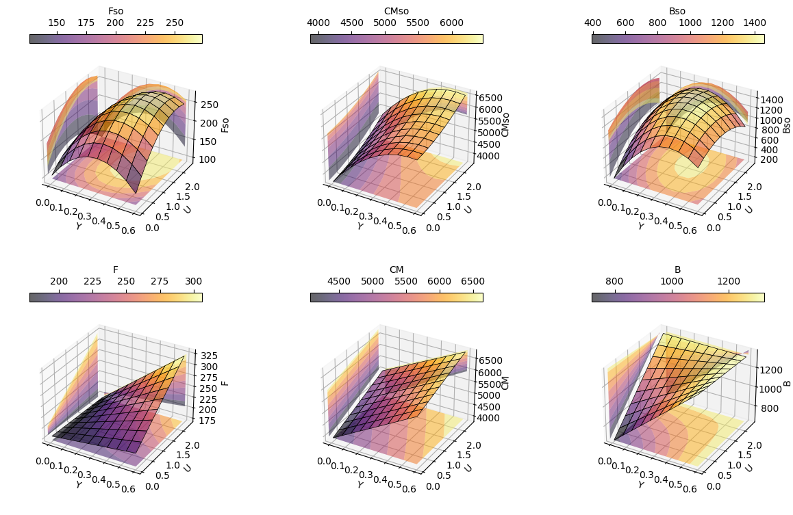
[148]:
fig, ax = plt.subplots(2,3, figsize=(15,9),subplot_kw={"projection": "3d"})
ax = ax.flatten()

for i,(key,val) in enumerate(fm_ccd.functions.items()):
    plot_surface(x='Y', y='U', z=key,
         model=fm_ccd,
         n_pts=10,
         ax=ax[i],
         other_params=dict(),
         labels=dict(xlabel='Y', ylabel='U', zlabel=key), cmap='inferno', scaled=True)
Optimization Using Desirabilty Function
A desirability function \(D\) is used to optimize the two independe variables at same time.
The function \(d_i\) was defined as
[285]:
@latexify.with_latex
def d_i(Y, Ymin=Ymin, Ymax=Ymax, r=1):
    if Y <= Ymin:
        return 0
    elif Y > Ymin and Y < Ymax:
        return ((Y-Ymin)/(Ymax-Ymin))**r
    else:
        return 1

d_i
[285]:
[269]:
from scipy.optimize import minimize
import latexify

responses = ['Fso','CMso','Bso']
model = fm_ccd
Ymax = 7000
Ymin = 200


def D(independent_vars):
    d_list = []
    for Yi in responses:
        d_list.append( d_i(model[Yi].predict(dict(U=independent_vars[0],Y=independent_vars[1]))[0]) )
    d_array = np.array(d_list)
    n = len(d_array)
    return 1-(np.prod(d_array)**(1/n))


from scipy import optimize as opt

x0 = (0, 0)
bounds = [(-1.41,1.41),(-1.41,1.41)]

optimum = minimize(D, x0, method='SLSQP', bounds=bounds)
optimum
[269]:
 message: Optimization terminated successfully
 success: True
  status: 0
     fun: 0.8802039525109903
       x: [ 6.344e-01  4.816e-01]
     nit: 10
     jac: [ 1.291e-04  2.973e-05]
    nfev: 30
    njev: 10
Anova table and lack of fit
To check model validity an ANOVA test and lack of fit can be used.
[270]:
fm_ccd.anova('Fso')
[270]:
| df | sum_sq | mean_sq | F | PR(>F) | |
|---|---|---|---|---|---|
| U | 1.0 | 3099.522852 | 3099.522852 | 4.600914 | 0.084782 |
| Y | 1.0 | 7419.724833 | 7419.724833 | 11.013797 | 0.021038 |
| U:Y | 1.0 | 1056.250000 | 1056.250000 | 1.567891 | 0.265894 |
| np.power(U, 2) | 1.0 | 918.771390 | 918.771390 | 1.363819 | 0.295530 |
| np.power(Y, 2) | 1.0 | 7192.080882 | 7192.080882 | 10.675884 | 0.022263 |
| Residual | 5.0 | 3368.377315 | 673.675463 | NaN | NaN |
[271]:
fm_ccd.lack_of_fit('Fso', alpha=0.05)
[271]:
| Source_of_Variation | df | sum_sq | mean_sq | F | F_table | p | |
|---|---|---|---|---|---|---|---|
| 0 | Regression | 3.0 | 11575.497685 | 3858.499228 | 2.352901 | 4.346831 | 0.158352 |
| 1 | Residual | 7.0 | 11479.229588 | 1639.889941 | NaN | NaN | NaN |
| 2 | Lack_of_Fit | 5.0 | 11297.229588 | 2259.445918 | 24.829076 | 19.296410 | 0.039167 |
| 3 | Pure_Error | 2.0 | 182.000000 | 91.000000 | NaN | NaN | NaN |
| 4 | Total | 10.0 | 23054.727273 | NaN | NaN | NaN | NaN |
Optmization Results
In the original papaer authors have found a desirability function of 0.87 and an optimum point at
The corresponding cellulase activities of
Totaling a production of 8085 U/L. In this work the desirabilty function was 0.88 and the optium point found at
This corresponts to a total cellulase activity of 8106 U/L, from which partial values for each metric are
[280]:
fm_ccd.decode_variables(variables=dict(U=optimum.x[0], Y=optimum.x[1]))
[280]:
{'U': 1.7069155936557219, 'Y': 0.39546634255213986}
[281]:
F=fm_ccd.predict(function='Fso', variables=fm_ccd.decode_variables(variables=dict(U=optimum.x[0], Y=optimum.x[1])))
F
[281]:
0    244.92823
dtype: float64
[282]:
C=fm_ccd.predict(function='CMso', variables=fm_ccd.decode_variables(variables=dict(U=optimum.x[0], Y=optimum.x[1])))
C
[282]:
0    6623.108285
dtype: float64
[283]:
B=fm_ccd.predict(function='Bso', variables=fm_ccd.decode_variables(variables=dict(U=optimum.x[0], Y=optimum.x[1])))
B
[283]:
0    1238.00179
dtype: float64